The first key component was concerned on defining the architecture of the data chain and starting processing archived imagery available in the Ny-Ålesund area. The selected datasets include the cameras operating at the Zeppelin Observatory [Pedersen, 2013], maintained by NPI, and the device supported by CNR at the Amundsen-Nobile Climate Change Tower [Salzano et al., 2022].
The pre-processing performed on the available imagery is focused on checking metadata associated with the image file, looking at the image size and the pixel resolution. Such a preliminary survey can identify failure in the data corruption and hopefully some issue in the server accessibility. The second step is the analysis of RGB values and their image patterns with the major goal to identify images characterized by low illumination, as well as situation with intense cloud cover. Finally, additional lens interferences (rain drops or ice crusts) are discarded.
The monoplotting of the image on the surface require two key information about the camera orientation and the sensor specifications. The preliminary process consists of calibrating the time-lapse camera using a reference chessboard. This operation is based on having at least 6 images shot by the camera system with the reference chessboard in a close-range distance. Having different chessboard orientations in front of the camera is possible, using standard computer vision techniques [Zhang, 2000], to obtain the intrinsic lens features useful for correcting the lens distortion.
The orthorectification module is based on the geometrical correction of the perspective view. This step is implemented following [Corripio, 2004]. The available digital elevation model [Porter et al., 2022], with a 5 m spatial resolution and 1 m vertical resolution, provided several topographic points that were projected on the camera view. The effectiveness of the correction was estimated considering the available ground control points.
The Segmentation procedure is based on the Spectral Similarity approach, proposed by [Salzano et al., 2019]. The module is based on measuring
the spectral variations in a 3D colour space where reference endmembers are a theoretical “white” snow and a theoretical “black” target. The
parameters estimated in this vector system are the spectral angle defined by [Kruse et al., 1993] and the Euclidean distance [Jensen, 2015],
respectively calculated considering white and black references. While the parameter based on the Spectral Similarity represents an independent
spectral feature, the Euclidean distance of the vector can be defined as a brightness-dependent feature. The involvement of all the three-color
components will support the increase of surface types that can be discriminated: snow, shadowed snow and not snow. The proposed approach was
developed in the R programming environment [R Core Team, 2022].
The first step consists of rearranging the three-color components of each pixel into a new two-dimensional vector space, mathematically
defined as follows: the spectral angle which represents the relative proportion of the three-pixel components in relationship to the reference
composition. The angle varies from zero, which can be associated with a “flat” behaviour of colours (R = G = B), to π2, referring to a very
dissimilar behaviour from the theoretical “white” reference. The spectral distance is conversely an estimation of the vector length in the RGB
space. It can range from 0 (black) to 1.73 (white) and it can be associated with the Euclidean distance from a “black” reference RGB composition.
While this parameter is sensitive to the brightness of colours, the spectral angle is invariant with brightness [Van der Meer, 2006].
The outcome of this step consists in the frequency counting of pixels considering the two spectral components with a 0.05 resolution.
Furthermore, the total number of included pixels and the area included in the cluster perimeter can be estimated.
The second step of the procedure consists in discriminating clusters from the obtained frequency distribution, and a watershed
algorithm [Vincent et al., 1991] can support this segmentation phase. Each cluster was fitted with a normal distribution to retrieve modes
and deviations. If clusters are very close to each other, they can be combined in one larger group depending on their probability to be
discriminated using the Mahalanobis distance. The criteria adopted for the definition of the cluster perimeter was based on the pixel frequency
higher than the Poisson error of the adjacent pixel. The procedure for the delimitation of the cluster perimeter was implemented using a
per-pixel method following [Seo et al., 2016].
The final step consists in the identification of the surface type (snow, not snow and shadowed snow). This step was defined observing the frequency distributions of pixels in the defined spectral space (Figure 1). It was possible to detect that snow covers were generally characterized by higher spectral angles and lower distance values than not-snow covers. Snowed centroids (defined by μΔ and μθ) were generally positioned where angles were higher than 0.9 and distances were lower than 0.1.
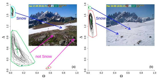 Figure 1. Examples of two different snow-not-snow mixtures [Salzano et al., 2019].
Coloured polygons identified areas of clusters in presence of two different situations: partial (a) and full (b) snow cover.
Lower plots are frequency distribution of pixels at the different spectral angles (θ) and spectral distances (Δ).
Figure 1. Examples of two different snow-not-snow mixtures [Salzano et al., 2019].
Coloured polygons identified areas of clusters in presence of two different situations: partial (a) and full (b) snow cover.
Lower plots are frequency distribution of pixels at the different spectral angles (θ) and spectral distances (Δ).
Combining the classification output with the ortho-projection procedure it is possible to prepare a product concerning the fractional
snow-covered area (FSCA). The grid extraction can be based on specific satellite products (Sentinel-2). The data format is the netCDF
standard format, where metadata is prepared following the ISO 19115 guidelines and the Climate & Forecast convention.
Read more ...
The chessboard calibration is a computer vision task that must be approached considering some guidelines:
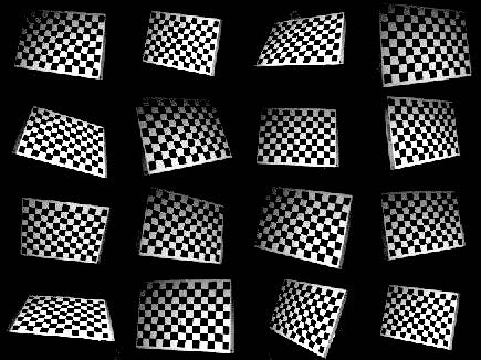
Figure 1. Examples of potential target orientations
